Predicting brain activity with Neural Nets and TensorFlow is easy(-ish)
Over-fitting is a lie.
Backgroud
I previously talked about predicting and decoding brain activity as recorded using fMRI. In that post I followed the tried and true approach of (1) extracting some features from the stimulus and (2) fitting a regularised linear regression from the features to brain activity. It works really well.
One of the reasons we use linear regression in these type of “encoding” studies is that there is not much data. For example in that study the training set had only about 7200 samples (which is quite a lot by fMRI community standards). The traditional thinking is that very rich models, such as deep neural nets (NNs) with millions of parameters, will disastrously over-fit in this type of situation, resulting in low performance. However, this traditional thinking may be out of date.
A recent paper uploaded to bioarxiv generated some discussion in our lab. It is a very thorough study looking at predicting brain activity using deep NNs with many interesting results. Among these results, the authors show that replacing the linear regression with a NN provides a substantial improvement over linear regression (see also here).
I think is pretty likely that with some effort and a lot of NN know-how an expert can improve on the performance of a linear model. But I figured that avoiding over-fitting in this situation is going to be really hard, and that an out of the box implementation would perform disastrously. So I thought I’d give it a go.
In this post I go through fitting a simple NN, though still with millions of parameters, to predict brain activity. I’ll use a vanilla NN paired with the same data I analyzed in my previous post. This way we will have a direct comparison with the linear model. A full notebook to reproduce this is up on my github.
Preparations
We will use the same data from last time. For convenience I put everything you’ll need here.
import numpy as np
import matplotlib.pyplot as plt
plt.rcParams["font.size"] = "20"

import tensorflow as tf
from tensorflow import keras
from tensorflow.keras import layers
from tensorflow.keras.callbacks import Callback
from tensorflow.keras import backend as K
#load the preproc data from before
with np.load("./data.npz") as f:
    print(f.files)
    voxel_test_data = f["voxel_test_data"]
    voxel_train_data = f["voxel_train_data"]
    ME_features_train_data = f["ME_features_train_data"]
    ME_features_test_data = f["ME_features_test_data"]
    linear_model_acc = f["linear_model_acc"]
- voxel_train_data this is the brain activity data we will use to train the model
- voxel_test_data this is the brain activity data we will use in the final test of the model
- ME_features_train_data this is the ME feature data we will use to train the model. The feature vector consists of stacking together four consecutive delays (t-3 to t-6, see the original post for details)
- ME_features_test_data this is the ME feature data we will use in the final test of the model
- linear_model_acc this is the accuracy data for the linear model. This is calculated as the pearsons correlation between the model predictions and the test data (i.e. voxel_test_data)
I restrict the analysis to the 2000 voxels that were best predicted using the linear model. This is a bit harsh on our NN here because it is possible that the NN improves on voxels that the linear model was poor at predicting, so keep that in mind.
feature_dim = ME_features_train_data.shape[1]
num_voxels = voxel_train_data.shape[1]
The network
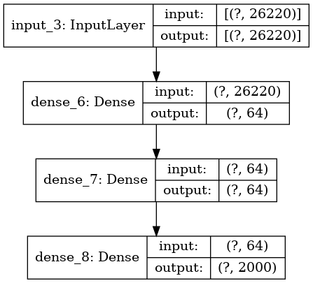
We first need to decide on the structure of the network. There is now a whole zoo of network architectures and I think it is pretty likely that many of them are superior to the linear model. However, the point here to see how well an “out of the box” NN works. Nothing is more vanilla than a tutorial, so I will use the architecture from the TensorFlow regression tutorial. The architecture has two hidden, densely connected layers with relu activations. We will be fitting a mere 1,812,304 parameters.
There really is no reason to think that this architecture is suited to our specific problem. But if something like this does work, then it may not be so difficult to come up with a NN that is superior to the linear model.
To the model.
# repeatable intialization of the weights
initializer = tf.keras.initializers.GlorotNormal(seed=1)

vanilla = tf.keras.Sequential([
    tf.keras.Input(shape=[feature_dim]),
    layers.Dense(64, activation='relu',kernel_initializer=initializer), # set the initial weights
    layers.Dense(64, activation='relu',kernel_initializer=initializer),
    layers.Dense(num_voxels)
])
vanilla.summary()
Model: "sequential_2"
_________________________________________________________________
Layer (type)                 Output Shape              Param #
=================================================================
dense_6 (Dense)              (None, 64)                1678144
_________________________________________________________________
dense_7 (Dense)              (None, 64)                4160
_________________________________________________________________
dense_8 (Dense)              (None, 2000)              130000
=================================================================
Total params: 1,812,304
Trainable params: 1,812,304
Non-trainable params: 0
_________________________________________________________________
keras.utils.plot_model(vanilla, show_shapes=True,to_file='vanilla.png')
The optimizer
The next thing is to choose an optimizer for the network. The tutorial used ADAM with a hardwired learning rate, but I went with a simple weight decay approach. Standard stuff, though I did manually tweak it a bit. A more principled approach is to optimize this using cross validation or something but for simplicity I’ll keep this as is.
# initial learning rate
initial_learning_rate = 0.0001
#expontential decay
lr_schedule = tf.keras.optimizers.schedules.ExponentialDecay(
initial_learning_rate,
decay_steps=1000,
decay_rate=0.8)
Compile
Put it all together
# optimize mean squared error
vanilla.compile(
    optimizer=tf.optimizers.Adam(learning_rate=lr_schedule),#
    loss='mean_squared_error',
    metrics=["mean_squared_error"])
Custom callback to monitor things
As I mentioned, the performance of the model is assess as the correlation between the predicted and actual response (more on this later). This will quickly evaluate our model performance
zs = lambda v,dim=0: (v-v.mean(dim,keepdims=True))/v.std(dim,keepdims=True)

def respective_correlation(x,y,dim=0):

    """
        shape is samps by vars/featurs
    """

    num_samps = x.shape[dim]
    if not np.array_equal(x.shape, y.shape):
        raise ValueError('x and y must have same shape')

    corrs = (zs(x,dim) * zs(y,dim)).mean(dim)

    return corrs
# We create a custom call back to report on how things are progressing in the end of each epoch
class CustomCallback(Callback):

    def __init__(self, val_data): # this gives us access to the validation data (see https://github.com/keras-team/keras/issues/10472 )
        super().__init__()
        self.validation_data = val_data

    def on_epoch_end(self, epoch, logs={}): # on the end of each training epoch get

        # the current learning rate
        current_lr = self.model.optimizer._decayed_lr('float32').numpy()

        # the correlation between the predicted and actual response
        for val in val_dataset: # calculate correlation on the validation data
            mdl_pred = self.model.predict(val[0])
            val_corr = np.mean(respective_correlation(mdl_pred, val[1].numpy()))

        # add it to the logs (not sure if this is the correct way to do it but it works)
        logs["val_corr"] = val_corr
        print(f"current lr {current_lr:.2E} corr {val_corr:.03f},\
        MSE {logs['val_mean_squared_error']:.06f}") #, loss {logs['val_loss']:.06f}
Prepare the training and validation data
I will keep some data aside for validation as we train the model. The key thing to remember here is that we are using time series data. This means that the data is not iid. If we just grabbed samples randomly for validation then there is a good chance that dependent samples will be in the training set. For example, we may end up with sample at t=n in the val set but t=n-1 in the training set. These are dependent, and in fact likely to be quite similar. In this case performance on the validation test will reflect something of double dipping and probably be much higher than what we get on the final test set.
I will very crudely grab three chunks of 200 samples at intervals of 2000, 4000 and 6000 samples. This is completely arbitrary and pretty poor practice. We did much better on the ridge regression in the previous post, but I think it is good enough for illustration. Note that we might have a bit of leakage (since the samples around these chunks are still in the training set), but I think it is not too much of a worry.
all_data_inds = np.arange(ME_features_train_data.shape[0])
#keep the first, take three, chunk_len samples long chunks for validation
chunk_len = 200
chunk_starts = np.array([2,4,6])*1000
chunk_ends = chunk_starts+chunk_len
val_inds = np.concatenate([np.arange(strt,stp) for strt,stp in zip(chunk_starts,chunk_ends)])
trn_inds = np.delete(all_data_inds,val_inds)
TensorFlow likes its data in a particular way. This is really irritating to me.
train_dataset = tf.data.Dataset.from_tensor_slices((ME_features_train_data[trn_inds,:], voxel_train_data[trn_inds,:]))
# organized in batches ofo 32 to update the gradients (I think this is default)
train_dataset = train_dataset.batch(32)

# Prepare the validation dataset
val_dataset = tf.data.Dataset.from_tensor_slices((ME_features_train_data[val_inds,:], voxel_train_data[val_inds,:]))

#For the validation I compute the correlation across the entire val data, i.e. one batch
val_dataset = val_dataset.batch(len(chunk_ends))
Fitting
callback = CustomCallback(val_dataset) # initialize the callback
history = vanilla.fit(train_dataset,callbacks=[callback],
    epochs=20,
    # suppress logging
    verbose=0,
    validation_data=val_dataset)
current lr 9.55E-05 corr 0.087,        MSE 0.918076
current lr 9.13E-05 corr 0.167,        MSE 0.888940
.
.
Plot the results
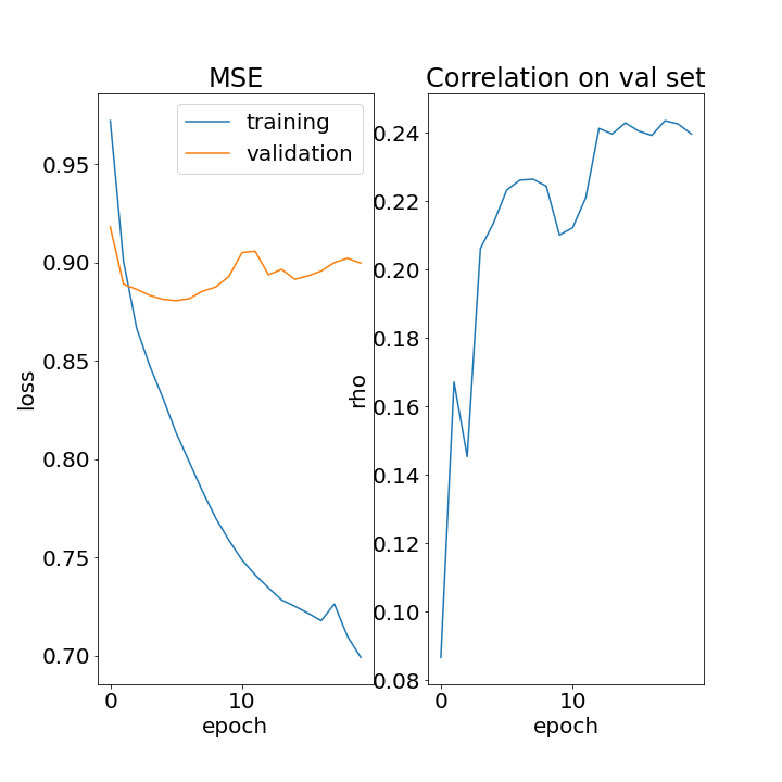
Pretty clear from above that the MSE continues to improve on the training set (blue, left panel) but validation performance is pretty much saturated after 1-2 epochs (orange, left panel). We’re over-fitting. A similar thing for the correlation (right panel). It improves a bit in the start but not too much happening after that. You are probably thinking that it is odd to fit using MSE as the loss and then use the correlation as the metric. You are right, but this is pretty common in encoding studies. The reason is that we usually use regularization, and this tends to reduce the norm of the prediction, producing pretty average MSE. However, the correlation between the predicated and actual response can still be high, indicating that the model has captured much of the temporal structure. So we use correlation to chose hyperparameters and assess the model but fit based on minimizing the MSE. Of course, here in TensorFlow, we could write a custom fit using pearson corr as the loss but that is a bit more advanced (I have actually done this and it works pretty well though the norms seem to explode, which is understandable. Anyhow, that’s for another time).
Compare with ridge
Let’s compare our results with the linear model. Based on our over-fitting above, I am expecting a complete disaster
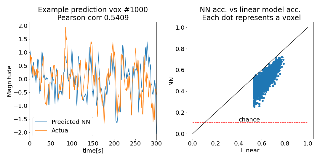
Well to my great surprise, our vanilla NN, with its millions of parameters trained on just thousands of samples, unquestionably works. Looking at the actual prediction for one voxel (#1000, left panel) we can clearly see that we captured much of the temporal structure - not too shabby!. Looking across all voxels (right panel), we see that the prediction accuracy for each voxel is far above chance (all voxels are far above the dashed chance level, which I estimated using a lazy permutation test. Check out the repo for details). Of course our linear solution is far superior (all voxels lie below the x=y line). One reason for this is that we optimized the regularization weights for the linear model whereas our NN is currently un-optimized.
A tinny bit of optimization
Let’s try to improve a bit with regularization. We will add a couple of dropout layers and also some L2 regularization. We will search through a grid and pick the combination with the best accuracy on the validation test.
HP_DROPOUT1 = np.linspace(0,0.8,5) # just 5 steps
HP_DROPOUT2 = HP_DROPOUT1.copy()
HP_L2_1 = np.linspace(0,.01,5)
HP_L2_2 = HP_L2_1.copy()
# a wrapper for constructing the network and fitting
def train_test_model(hparams):

    tmp = tf.keras.Sequential([
        tf.keras.Input(shape=[feature_dim]),
        layers.Dropout(hparams["HP_DROPOUT1"]),
        layers.Dense(64, activation='relu',kernel_initializer=initializer
                     ,kernel_regularizer=tf.keras.regularizers.l2(hparams["HP_L2_1"])),
        layers.Dropout(hparams["HP_DROPOUT2"]),
        layers.Dense(64, activation='relu',kernel_initializer=initializer,
                     kernel_regularizer=tf.keras.regularizers.l2(hparams["HP_L2_2"])),
        layers.Dense(num_voxels)
    ])

  # optimize mean squared error
    tmp.compile(
    optimizer=tf.optimizers.Adam(learning_rate=lr_schedule),#
    loss='mean_squared_error',
    metrics=["mean_squared_error"]
    )

    callback = CustomCallback(val_dataset) # initialize the callback
    history = tmp.fit(train_dataset,callbacks=[callback],
        epochs=5, #keep this low, otherwise it takes too long
        # suppress logging
        verbose=0,
        validation_data=val_dataset
                         )

    return history.history["val_corr"][-1]
# well I admit these loops took loner than I thought (~4 hours on my CPU only version of tf) so you may want to dial it down a touch
opt_results = []
for dropout_rate1 in HP_DROPOUT1:
    for dropout_rate2 in HP_DROPOUT2:
        for l2_1 in HP_L2_1:
            for l2_2 in HP_L2_2:
                hparams = {
                    'HP_DROPOUT1': dropout_rate1,
                    'HP_DROPOUT2': dropout_rate2,
                    'HP_L2_1': l2_1,
                    'HP_L2_2': l2_2,
                }

                print(hparams)
                this_res = train_test_model(hparams)
                opt_results.append([hparams,this_res])
{'HP_DROPOUT1': 0.0, 'HP_DROPOUT2': 0.0, 'HP_L2_1': 0.0, 'HP_L2_2': 0.0}
current lr 9.55E-05 corr 0.069,        MSE 0.916014
current lr 9.13E-05 corr 0.144,        MSE 0.889414
.
.
Get the best performing params
opt_params,opt_corr = zip(*opt_results)#
opt_corr = np.array(opt_corr)
argsortres = np.argsort(opt_corr)
top_params = opt_params[argsortres[-1]]
Fit the entire training set with the optimized params. Btw, these were the values I got {‘HP_DROPOUT1’: 0.275, ‘HP_DROPOUT2’: 0.275, ‘HP_L2_1’: 0.007750000000000001, ‘HP_L2_2’: 0.007750000000000001}
top_params = {'HP_DROPOUT1': 0.275, 'HP_DROPOUT2': 0.275, 'HP_L2_1': 0.007750000000000001, 'HP_L2_2': 0.007750000000000001}
vanilla_opt = tf.keras.Sequential([
        tf.keras.Input(shape=[feature_dim]),
        layers.Dropout(top_params["HP_DROPOUT1"]),
        layers.Dense(64, activation='relu',kernel_initializer=initializer
                     ,kernel_regularizer=tf.keras.regularizers.l2(top_params["HP_L2_1"])),
        layers.Dropout(top_params["HP_DROPOUT2"]),
        layers.Dense(64, activation='relu',kernel_initializer=initializer,
                     kernel_regularizer=tf.keras.regularizers.l2(top_params["HP_L2_2"])),
        layers.Dense(num_voxels)
    ])

# optimize mean squared error
vanilla_opt.compile(
optimizer=tf.optimizers.Adam(learning_rate=lr_schedule),#
loss='mean_squared_error',
metrics=["mean_squared_error"]
)

vanilla_opt_history = vanilla_opt.fit(ME_features_train_data,voxel_train_data,
    epochs=100,
    verbose=1,# just to see how things are progressing
    validation_data=0
                     )
Epoch 1/100
223/223 [==============================] - 2s 8ms/step - loss: 1.9031 - mean_squared_error: 0.9528
Epoch 2/100
223/223 [==============================] - 2s 8ms/step - loss: 1.3411 - mean_squared_error: 0.8756
.
.
.
# Our optimized predictions
preds = vanilla_opt.predict(ME_features_test_data)
NN_corrs_opt= respective_correlation(preds,voxel_test_data)
Let’s have a look
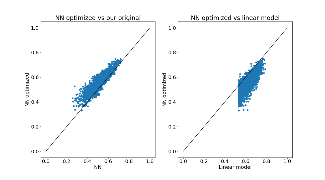
So we can see the optimization improves on our original effort (almost all voxel are above x=y line, left panel), as expected. However, as compared to the linear model, our NN is still doing worse (most voxels below x=y line, right panel).
Final thoughts
It turns out that it is possible to train a vanilla neural network with millions of parameters to predict BOLD activity using just thousands of training samples, and yet do a reasonable job. We performed far better than chance. In our case we cannot beat the linear model, but there are some things to keep in mind here. First, our NN architecture is completely arbitrary and almost certainly not ideal for this type of task. Second, we chose the best voxels according to the linear model, so the comparison is a bit skewed in its favor. Third, our linear model is not vanilla, in the sense that it sits at the end of a pipeline designed to make it work (that is to say that there is a long history of fitting linear models to predict BOLD data and I drew on that to build it. There is much less out on fitting NNs for this kind of thing, so less prior knowledge). Lastly, in the linear approach we optimized the regularization for each voxel separately, and then fit each voxel separately. In that sense, our linear model actually has (26220=feature dim)x(2000=num voxels)+(2000=num hyper params) = 52,442,000 parameters, which is much more than our NN, which only had 1,812,304 parameters. In the NN here we fitted all 2000 simultaneously, simply by changing the output of the top layer. So there is a qualitative difference here that deserves a bit more scrutiny. All in all, I am pretty confident that if these differences were addressed we could match and improve on the linear model.
The point here, however, was to see how difficult it would be to fit a NN with millions of parameters to a “typical” encoding data set, which usually only has thousands of samples per voxel. It turns out that even an “out of the box” vanilla implementation works pretty well. One advantage of the TensorFlow setup is that once the basic fitting code is in place, it is very easy to try different variations. Adding and dropping layers, trying different activations and regularizations is a breeze. Tip of the hat to the NN community for developing these unbelievable tools. I think in the future I will run something like this along my standard workflow just to see what it looks like. Maybe in time it will become my go-to. Who knows.
At the start of the post I said that one of the reasons we don’t use NNs is that fitting them is difficult. Well, as we see here, that argument may not be a very good one. But there are other reasons to use linear models. For example, they are easy to fit (e.g. linear regression + L2 has an analytic solution), well understood (e.g. bias and avariance trade off, statistical tests) and, clearly, do quite well. Most importantly, they are transparent and easy to interpret. The prediction is just a linear sum of the features. This is critical in neuroscience where we don’t just want to predict, we want to understand.